Credit Decision Engine

This credit decision engine predicts when borrowers default with a discrete-time competing-risks hazard model, calibrates those probabilities well enough to price a loan with, and wraps them in an approval rule that maximises expected profit rather than accuracy. It is not a default classifier: the target is a decision, and the probability of default is an input to it rather than the output of the exercise.

Technical terms are marked * at first use and collected in the glossary at the end.

Overview

A lender approving a loan is deciding whether the expected discounted cash flow from an applicant exceeds the capital it ties up. Most public credit-risk work stops well short of that, instead fitting a classifier to a binary "did this default" target, then reporting AUC*, and finally picking a threshold near where accuracy peaks. Three things are wrong with that, and this project is built to measure each one.

1. Timing matters as much as incidence. A binary target discards the timing, and with it most of the economic content. A loan defaulting in month 2 destroys far more value than one defaulting in month 30, because in the second case 28 payments have been collected.
2. Level matters more than ranking. An NPV calculation consumes the probability of default, not the ranking, whereas AUC only sees ranking, meaning an excellent AUC with systematic overconfidence still misprices every loan in the book.
3. The optimal cutoff is an economic quantity, not a statistical one. A threshold based on accuracy or F1 is built on the ratio of right and wrong predictions, not taking into account the possible losses or gains of each loan. The optimal cutoff should be calculated per loan to maximise expected profit.

Overarching Theory

The whole engine is based on the equation for Net Present Value (NPV)* which describes how profitable an investment will be by comparing the present value of future cash flow to the investment's cost. It has the following general form, which sums every future cash flow, each discounted back to what it is worth today, then subtracts the money put in at the start:

$$\text{NPV} = \sum_{t=1}^{N}\frac{C_t}{(1+i)^{t}} - \text{initial investment}$$

where

• $C_t$ is the cash flow in period $t$,
• $i$ is the required return, or discount rate*, the rate at which a future pound is worth less than one today, because a pound now can be put to work (for a lender, it reduces what must be borrowed to fund the loan),
• $t$ is the number of time periods, running to the final period $N$.

The factor $1/(1+i)^t$ is the discount factor*: it shrinks a pound arriving in $t$ periods to its value now. This is the textbook formula for any investment whose cash flows are known, such as a bond, a project, or a savings plan. A loan almost fits the equation except that its cash flows are not known, because the borrower may stop paying at any point.

The rest of this section is the sequence of steps that turns the general formula into one that handles that uncertainty.

1. Put the general terms into loan language.

The initial investment is the principal* $P$, the money lent at origination, the only negative term. The discount rate $i$ becomes a monthly rate $r$, and the period $t$ counts months on book.

2. The monthly cash flow is uncertain, so $C_t$ becomes an expected cash flow.

This is the whole difference between a loan and a bond. In the general formula $C_t$ is a fixed, known number. The amount of cash repayed in month $t$ is random since the borrower can do multiple things: pay as scheduled, repay the loan early, or might default. So $C_t$ is replaced by its statistical expected value. Computing that expectation is what steps 3 to 5 do; once we have it, we simply substitute it back into the general formula.

3. Enumerate each scenario that can happen, and the cash each pays.

In any month a live loan does exactly one of three things:

• defaults: stops paying; you recover only part of the balance, $B(t)(1-\text{LGD})$, where LGD* (loss given default) is the fraction of the balance you fail to recover;
• prepays: repays its entire outstanding balance $B(t)$ early and terminates. You get your money back, but forgo all future interest;
• performs: pays the scheduled amount $M$ and continues.

Here $B(t)$ is the balance still owed at month $t$, which falls as principal is repaid. Because the outcomes are exclusive, in a month the loan exits it pays the balance or the recovery, not $M$ as well.

4. Attach a probability to each outcome: hazards.

Conditional on the loan being alive at the start of month $t$, we define

• $h_d(t)$, the probability it defaults this month,
• $h_p(t)$, the probability it prepays this month,
• $1 - h_d(t) - h_p(t)$, the probability it performs and survives to the next month.

Each is a hazard*, defined as the chance an event strikes this month given the loan reached this month. Producing these two curves (one per hazard) per loan is the model's entire job (Stage 2). Weighting each outcome's cash by its probability gives the expected cash for a loan known to be alive at month $t$:

$$\underbrace{\big(1 - h_d(t) - h_p(t)\big)\,M}_{\text{performs}} \;+\; \underbrace{h_p(t)\,B(t)}_{\text{prepays}} \;+\; \underbrace{h_d(t)\,B(t)(1-\text{LGD})}_{\text{defaults}}$$

5. Calculate the chance the loan is alive at all.

Step 4 assumed the loan reaches month $t$ alive. The probability of that is the chance it survived every earlier month, which is the running product of the monthly survival probabilities and is given by the survival function* $S(t)$:

$$S(t) = \prod_{u<t}\big(1 - h_d(u) - h_p(u)\big)$$

6. Form the NPV expression.

A loan that has already exited, with probability $1 - S(t)$, pays nothing more. Therefore in month $t$:

$$\begin{aligned} \text{expected cash} &= (\text{prob. alive}) \times (\text{expected cash given alive}) + (\text{prob. exited}) \times 0 \\[2pt] &= (\text{prob. alive}) \times (\text{the expression in step 4}) \\[2pt] &= S(t)\big[\big(1 - h_d(t) - h_p(t)\big)\,M \;+\; h_p(t)\,B(t) \;+\; h_d(t)\,B(t)(1-\text{LGD})\big] \end{aligned}$$

The result. Substituting this expected cash flow back into the general formula in place of $C_t$, with $P$ for the initial investment and $r$ for $i$, gives the identity the project runs on:

$$\text{NPV} = -P + \sum_{t}\frac{S(t)\big[\big(1 - h_d(t) - h_p(t)\big)\,M \;+\; h_p(t)\,B(t) \;+\; h_d(t)\,B(t)(1-\text{LGD})\big]}{(1+r)^{t}}$$

The equation shows where the project's claims live: timing enters through $S(t)$ and the discount factor (a loss in month 2 and the same loss in month 30 discount to very different values), while the level of the probabilities enters through $h_d(t)$.

How the equation is used in the project

This single identity is what ties the stages together, and each stage supplies or stresses one piece of it:

• Stage 2 produces the hazards $h_d(t)$, $h_p(t)$ per loan. These are the only model outputs; everything else in the equation is arithmetic or a measured assumption.
• Stage 3 checks those hazards are right as numbers, not just correctly ordered, because a well-ranking but mis-levelled hazard still prices every loan wrong.
• The economic inputs $r$, LGD, and the recovery lag are measured or bracketed from the data and sensitivity-swept*, never rounded. LGD is measured as an effective figure, $P(\text{loss} \mid \text{90+ DPD}) \times \text{severity}^{\text{*}} = 0.3697 \times 0.3596 \approx 0.1330$, because most borrowers who fall 90 days behind recover and cause no loss.
• Stage 4 turns the equation into the decision. Approve a loan if and only if its expected NPV is positive. There is no threshold to tune, only a value to compute and a sign to check.
• Finally, expected NPV makes each decision, but each decision is scored on realised cash* rebuilt from the loan's actual balance path, never on the forecast that made it, since that would grade an overconfident model with its own optimistic answer key. Stage 5's out-of-time* ablation* runs entirely on that realised cash.

Data

The dataset used: Freddie Mac Single-Family Loan-Level Dataset, Release 47 (July 2026), with ~49.2M originations and ~2.9Bn monthly performance records, January 1999 to March 2026. This project uses the 50,000-loans-per-vintage* random samples: 2000–2004 to train, 2006–2008 to test, an out-of-time split across the financial crisis, with 2005 omitted as the ambiguous transition year. That is 400,000 loans and 19.20M person-period* rows after a 120-month administrative censor*.

The data is not in this repo and never will be. It is licensed for use, not redistribution. Access is free but requires a Clarity Data Intelligence account, CRT portal (not MBS): https://claritydownload.fmapps.freddiemac.com/CRT/#/sflld → Data Download → SFLLD. Take sample_YYYY.zip for each vintage into data/raw/. The one committed data file is the FRED Treasury series behind the discount rate, which is US federal government work in the public domain.

Pipeline Structure

Stage	What it does	Code
1	Parse the pipe-delimited files against an explicit Release 47 schema into DuckDB; build the person-period table (one row per loan per month at risk); compute vintage curves in SQL	data/, features/
2	Fit cause-specific discrete-time hazards: logistic regression on person-period rows, loan age through a spline basis*, default and prepayment as competing causes*	models/
3	Measure calibration* (reliability, Brier, ECE)* in-sample, on an in-time holdout and out of time; recalibrate with Platt and isotonic*; price the difference	calibration/
4	Project loan NPV under the fitted hazards, rebuild realised cash from the observed balance path, and sweep the approval cutoff	economics/
5	The B0–B4 ablation on one out-of-time population, plus failure analysis by cohort and by risk decile	eval/

Results

All figures below are out-of-time. Section references are to PROJECT_PLAN.md.

Calibration holds in time and breaks out of time (§6c)

The table reports predicted defaults ÷ observed defaults. A ratio below 1 means the model predicts fewer defaults than actually occur; at 0.3717 out of time it predicts about a third of them.

Population	Rows	Default events	Predicted ÷ observed
train, in-sample (the fitted 80%)	9,691,658	7,416	0.9996
holdout, in-time (the unseen 20%)	2,427,055	1,834	1.0212
test, out-of-time (2006–2008)	7,082,483	18,978	0.3717

The in-time holdout at 1.0212 says overfitting accounts for about two percentage points and essentially nothing else, so the 0.3717 is a regime change rather than a generalisation failure. The ranking survives it intact, with the observed default rate rising monotonically across all twenty predicted-risk bins, while the level fails as an arch: calibrated at the safe end, worst in the middle, recovering somewhat at the risky end. Grouping the out-of-time book into twenty equal-count bins by predicted risk:

Predicted-risk bin	Observed ÷ predicted
safest	0.97×
middle	4.10×
riskiest	1.38×

The middle bins are off by more than 4×, and the middle is exactly where the approve-or-decline population sits, so the error is largest precisely where the cutoff has to be placed.

The cutoff is worth more than the model (§6d)

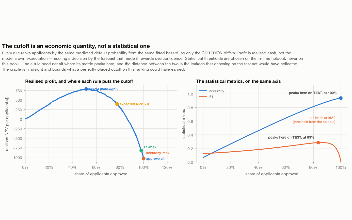
Every rule below ranks applicants by the same predicted 36-month default probability from the same fitted hazard, so only the criterion turning that score into a cutoff differs. Scored on realised cash. The oracle* is the best cutoff choosable knowing the result of each loan, not a number the lender can produce, but the ceiling that makes the other gaps interpretable.

Rule	Approves	Realised NPV per applicant
approve all	100.0%	−$1,034
accuracy-maximising	100.0%	−$1,034
F1-maximising (weighs misses and false alarms equally)	98.0%	−$824
expected NPV > 0	77.5%	+$393
oracle (hindsight)	51.5%	+$784

The accuracy-maximising cutoff is the same as the approve all rule, and by arithmetic rather than accident. At a 36-month default rate of 6.4% the true negatives dominate, so always approving will maximise accuracy due to this huge imbalance of defaulted loans.

Approving on positive expected NPV instead earns +$1,427 per applicant relative to the approve all and accuracy-maximising rules.

Calibration pays through where the cutoff lands, not through the portfolio total. Reading the probabilities at face value, the raw model approves 85% of the loans when about 63% was optimal, under-predicting default, so too many loans clear the "NPV > 0" bar. Calibrating the level shrinks those inflated NPVs, moving approval down to 71.5%. That single move is worth a further +$277 per applicant.

Capture* is defined as (what your rule earned) / (what the oracle earned). The raw rule captured 71.9% of the oracle's value, whereas post-calibration evaluation saw this rise to 95.5%.

The ablation (§6e)

An ablation stacks models so each one differs from the one above it by a single design choice, then scores them all identically so that any change in profit can be attributed to the singular choice and nothing else. This is how the project decomposes where the value actually comes from.

Every arm runs on the same 87,854 out-of-time applicants (the 2007–2008 loans) under the same economics, and the binary comparison model is handed the identical training loans, covariates, encoding and optimiser settings as the hazard. 85 features against 92, the missing 7 being exactly the loan-age spline columns the binary model has no time axis to use.

Two columns are the most important: Step is what each arm adds over the one directly above it. Its own forecast is what that arm expected to earn, shown to contrast with the value it realised.

arm	approves	realised	step	its own forecast	AUC
B0 approve all	100.0%	−$79	—	—	0.500
B1 binary, accuracy-max	100.0%	−$79	$0	$4,405	0.741
B2 binary, profit-max	89.2%	+$460	+$538	$4,541	0.741
B3 hazard, profit-max	84.5%	+$915	+$455	$3,640	0.806
B4a + in-time recalibration	84.7%	+$896	−$18	$3,652	0.806
B4b + sequential recalibration	71.3%	+$1,460	+$563	$2,660	0.803

Reading the table we see that B0 is the floor: approve everyone, no model, at −$79. As seen above, B1 has no effect on the realised value and B2 increases the realised NPV due to maximising profit over accuracy. This verifies Claim 3 made in the overview section. B3 then changes only the model, swapping the binary target for the discrete-time hazard. This adds a further +$455, additionally increasing AUC from 0.741 → 0.806. Knowing when a loan defaults improves the ranking as well as the pricing, which is more than Claim 1 strictly promised. B4a then recalibrates on held-back training data, the arm a lender could actually run, losing $18, doing nothing as stage 3 predicted, because in-time the model is already right and the recalibrator has nothing to learn. B4b recalibrates instead on the first test cohort's realised outcomes and is worth +$563, but that cohort takes 120 months to observe, so it is a ceiling on what recalibration could be worth, showing the possible maximised outcome.

The forecast (how much the model predicts to make) falls from $4,541 → $2,660 while the realised results (how much the model actually made) rise from $460 → $1,460. This is because as the model becomes better it becomes less overconfident, meaning that its forecast approaches the realised result which increases itself due to the model improving.

(Approve-all reads −$79 here against −$1,034 in §6d because this table drops the 2006 cohort, which is spent fitting B4b's calibrator; every arm is scored on the same 2007–2008 set.)

Where the model fails

We see that the model fails to predict the NPV of loans written in 2007 but succeeds in loans written in 2008: −$3,274 realised against +$2,854, on expectations of $733 and $5,838. This is because a 2007 origination met the financial crash about eighteen months in, near the hazard's peak with almost no principal amortised*, whereas a 2008 origination was written after prices had begun falling, under tighter underwriting. The difference between the loans is not their origination data but the timing of them meeting the financial crisis.

By comparing risk deciles*, we see that the error in prediction is a shape error rather than a level error. The expected vs realised gap varies elevenfold from safest to riskiest loan, which is why a two-parameter monotone recalibration* cannot fix it. Additionally, the model's expected NPV is positive in every decile while realised value crosses zero between the fifth and sixth, meaning a lender running it would see every segment profitable.

Underneath all of it is one structural limit. You cannot tell a loan's age apart from the calendar date and the cohort it came from, because any two of the three fix the third exactly ($\text{period} = \text{cohort} + \text{age}$). This is the age–period–cohort* identification problem, and no amount of data or spline flexibility escapes it. Origination covariates simply cannot represent a macro effect that is defined by the calendar. The same limit is behind the 2004 cohort's residuals in stage 2, the control arm under-predicting a book that looked safer at origination, and the 2007-versus-2008 gap above.

How much of the error is due to the crisis?

To answer this question we re-run with the break taken out of the comparison, training on 2000–2002 and testing on 2003–2004, keeping every assumption copied verbatim. The same experiment gives an NPV effect eleven times smaller (−0.061% against −0.693% of principal). This implies that the shape error magnitudes here are a result of the crisis and should not be quoted as typical.

What causes failure in both calm and crisis arms is the mechanism: the ranking holds while the level fails, in-time recalibration detects neither, and only recalibrating on the nearest out-of-time cohort helps. So the claim that generalises is not "calibration fails by 40% out of time" (the crisis) but "the same calibration does not transfer across time." The control can even date its own break since the cumulative default is calibrated to within 0.1% at 24 months but degrades significantly to 0.667 by 60 months. A 2003–2004 loan reaches 24 months in 2005–2006 and 60 months in 2008–2009, so the accuracy fails exactly as the crisis enters the test cohorts, not gradually with horizon.

Limitations

Design constraints rather than retrofitted analysis; PROJECT_PLAN.md §8 carries all thirteen with their measurements.

• The largest NPV magnitudes are from a crisis: Measuring across the 2008 crisis gives an effect 11 times larger than over a calm period. The mechanism, however, generalises but the magnitude does not.
• Selection bias cannot be corrected here: The population is made up of only approved loans, loans that passed an originator's underwriting and Freddie Mac's purchase criteria. This pushes estimates optimistic. The Standard dataset also excludes the worst-rated mortgages, namely Alt-A, no-doc and option ARMs, so the crisis degradation measured here is a lower bound on what the market suffered.
• Secured, not unsecured; US, not UK. Mortgage LGD is collateral-driven, unsecured consumer LGD is near-total. The regulatory and macro regimes differ meaning that the techniques used in this model can be carried over to different types of loans, but the numbers cannot.
• Default is first passage to 90+ DPD*, which is not a loss event. 63% of these loans recover and do not produce a loss disposition*. The model handles this through an effective LGD*, but the NPV cannot represent timing. This understates a loan's value by about 4.7% of its outstanding balance. A multi-state model is the correct treatment and the most valuable extension available.
• The terminal balance is booked at par* at the 120-month horizon, where 16.3% of principal has been repaid, because projecting hazards past the model's support would be inventing data. It cancels in the differences the results rest on, so there is no absolute NPV valuation.
• Censoring at 120 months captures 92.5% of eventual loss dispositions and misses 7.5%, leaving realised NPV optimistic by roughly $350 a loan.
• Oracle rows are hindsight, included only to bound what a ranking could have earned with a perfectly placed cutoff.

Out of scope, with reasons in §11: deployment or serving, deep learning, gradient boosting as the headline model, fair-lending analysis, and risk-based pricing with adverse selection.

Figures

Every panel below is out of time unless it says otherwise, and all six are regenerable from the CLI. Section markers point back to the results above.

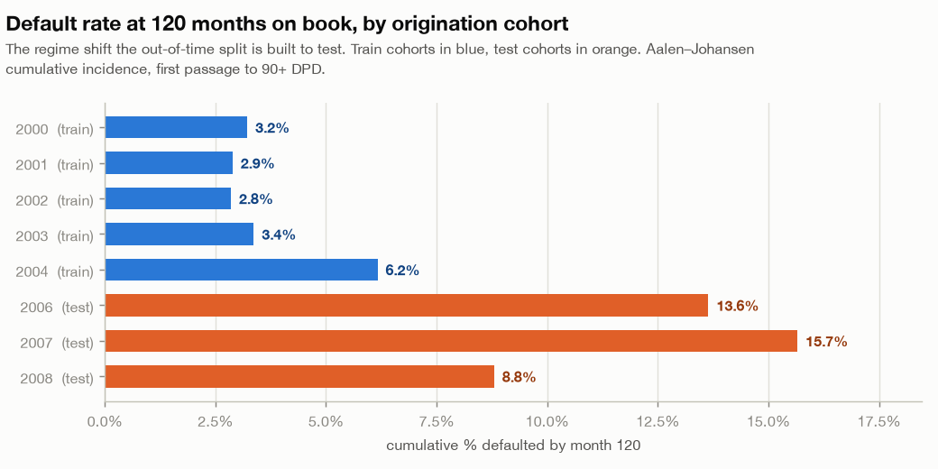
Figure 1. Cumulative default rate at 120 months on book, by origination cohort. Train cohorts run 2.8% to 6.2%, test cohorts 8.8% to 15.7%: the regime shift the out-of-time split is built to test.

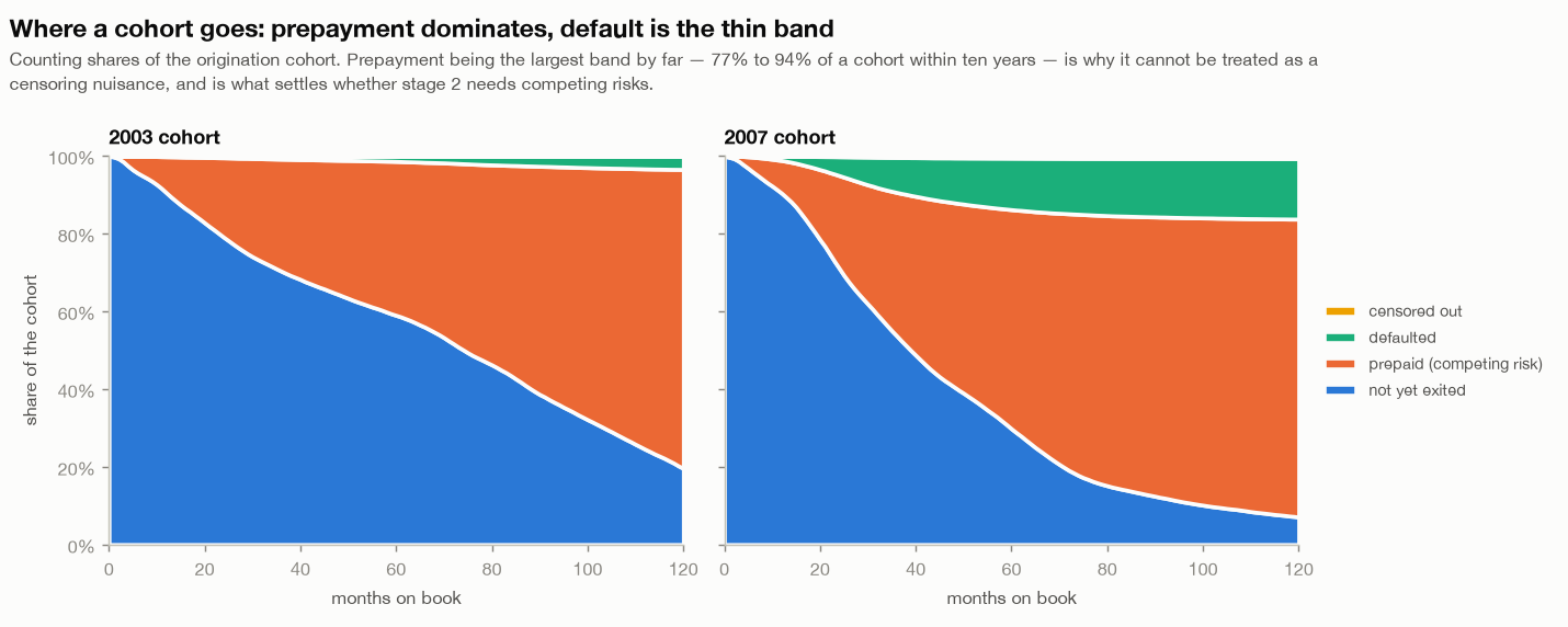
Figure 2. Where a cohort goes over ten years, for 2003 and 2007. Prepayment takes 77% to 94% of a cohort, which is why it has to be modelled as a competing risk rather than treated as censoring.

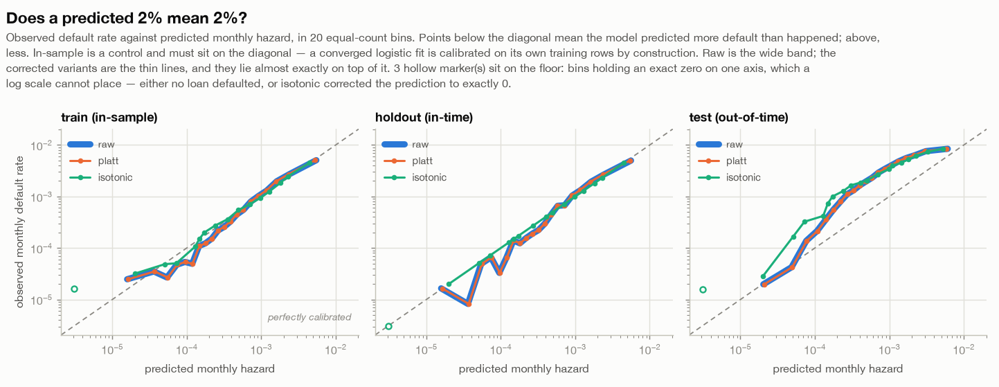
Figure 3. Observed against predicted monthly hazard, twenty equal-count bins, on all three populations (§6c). The first two panels sit on the diagonal and the out-of-time panel does not. Platt and isotonic lie almost on top of the raw curve, because both were fitted in time.

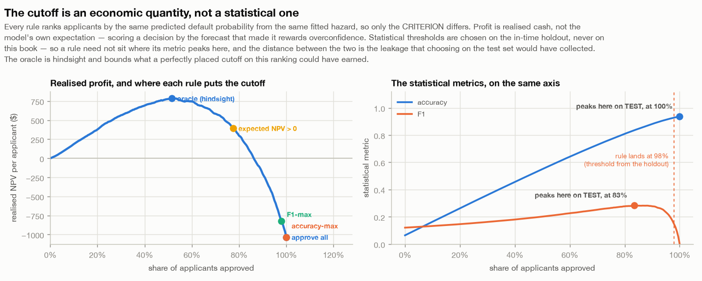
Figure 4. Realised profit per applicant against share approved, with each rule marked (§6d). Profit peaks near 50% approval while every statistical rule lands at 98% or above.

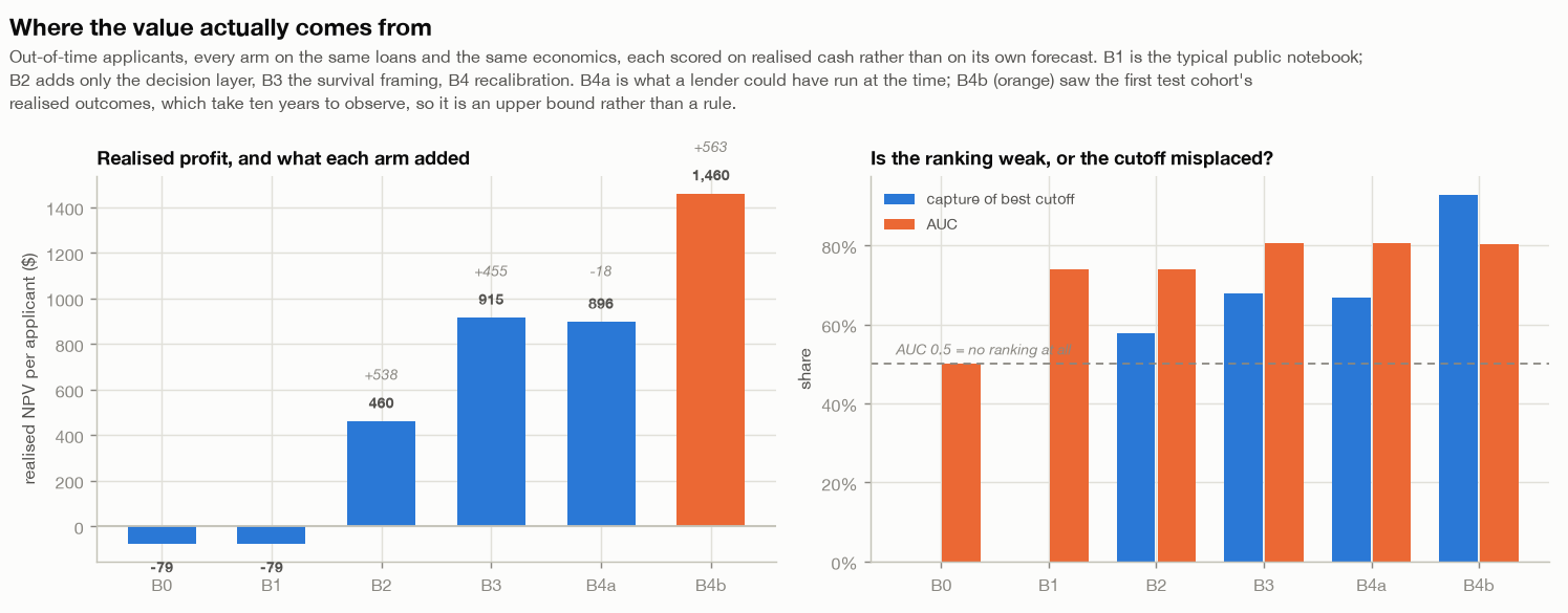
Figure 5. Realised profit by ablation arm, with the step each one adds, beside capture against AUC (§6e). B4b is drawn in orange because it saw the first test cohort's realised outcomes, which take 120 months to observe.

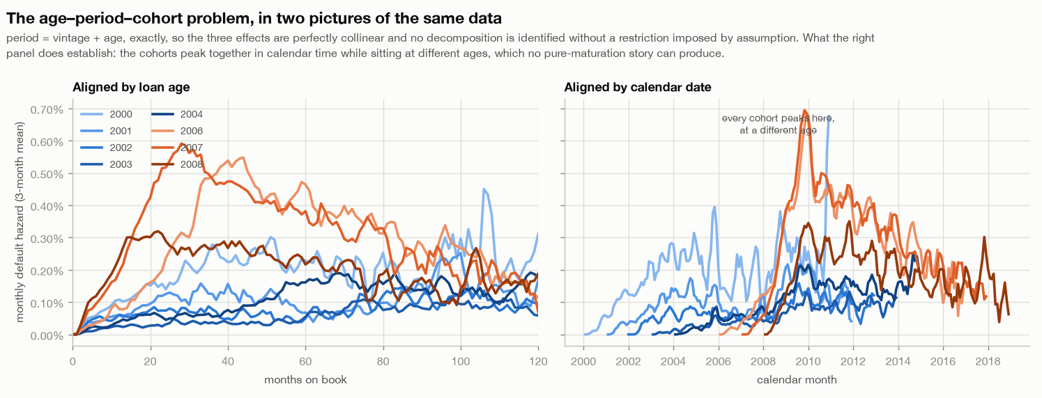
Figure 6. The same hazard data aligned by loan age and by calendar date. Every cohort peaks at the same calendar month at a different age, which no pure-maturation story can produce.

Glossary

Every term marked * in the text appears below, with the meaning it carries in this report rather than its most general one.

Term	Meaning
Hazard, $h(t)$	Given a loan was alive entering month $t$, the probability it defaults during month $t$. A per-month risk, not a cumulative one
Survival, $S(t)$	Probability a loan reaches month $t$ without leaving for any reason
Person-period data	One row per loan per month, the layout that lets ordinary logistic regression estimate a hazard
Competing risk	A rival exit that makes the event impossible afterwards. Prepayment is one: a repaid loan can never default
Censoring	Losing sight of a loan while it is still at risk. Missing information, not an outcome
PD / LGD / EAD	Probability of Default / Loss Given Default (fraction of money lost) / Exposure At Default (balance outstanding at that moment)
90+ DPD	90 or more days past due, meaning three missed payments, and the standard regulatory reference point for default
Vintage / cohort	The batch of loans originated in a given period
Age–period–cohort problem	Loan age, cohort quality and the calendar cannot be separated, because $\text{period} = \text{cohort} + \text{age}$ exactly
Net present value (NPV)	What an investment is worth today: every future cash flow discounted back to the present, minus the money put in at the start. Positive means it beats the required return
Principal, $P$	The money handed over at origination. The only negative term in the NPV identity
Discount rate, $i$ (monthly $r$)	The required return, so the rate at which a pound arriving later is worth less than one today
Discount factor	$1/(1+i)^t$, the multiplier that converts a pound arriving in $t$ periods into its value now
Severity	How much of a loan's balance is actually lost once it does go bad, 0.3596 here. Separate from how often that happens
Effective LGD	Severity scaled by the share of 90+ DPD loans that go on to produce a loss (0.3697), giving 0.1330. It lets a first-passage default target price as though it were a loss target
Loss disposition	The point at which a defaulted loan is finally resolved and the loss is booked
Amortisation	The repayment of principal over a loan's life. A loan that defaults early has amortised little, so more balance is still at risk
Par	Full face value. Booking the terminal balance at par values it at the amount outstanding rather than projecting hazards past the model's support
Realised cash	Cash rebuilt from a loan's observed balance path, so what actually happened. Decisions are scored on this, never on the forecast that made them
Spline basis	A set of columns that lets loan age enter the model as a flexible curve rather than a straight line
Calibration	Whether predicted probabilities are right as levels, not merely in the right order. A predicted 2% should mean 2%
Reliability, Brier, ECE	Calibration diagnostics. A reliability curve plots observed against predicted; the Brier score is mean squared error on probabilities; ECE is expected calibration error, the average gap between predicted and observed across bins
Platt / isotonic	Two recalibrators fitted after the model. Platt is a two-parameter logistic squeeze; isotonic is a free monotone step function
Monotone recalibration	Any correction that rescales probabilities while preserving their order. It can fix a level error, but not a shape error that varies across the risk range
AUC	Area under the ROC curve: the probability a random defaulter is ranked riskier than a random non-defaulter. It sees ranking only, never level
In-sample / in-time holdout / out-of-time	The three populations. In-sample is the rows the model was fitted on; the in-time holdout is unseen loans from the same vintages; out-of-time is later vintages, here on the far side of the crisis
Sensitivity sweep	Re-running the whole pipeline across a range of plausible values for an input, to see which results hold steady and which move with the assumption
Ablation	A stack of models where each differs from the one above by a single design choice, all scored identically, so any change in profit is attributable to that one choice
Oracle	The best cutoff choosable with hindsight. Not available to a lender, but it bounds what the ranking could have earned
Capture	What a rule earned divided by what the oracle earned
Risk decile	One tenth of the book, ordered by predicted risk